The Klein Gordon Field

2.1 The Necessity of the Field Viewpoint
13P4E5
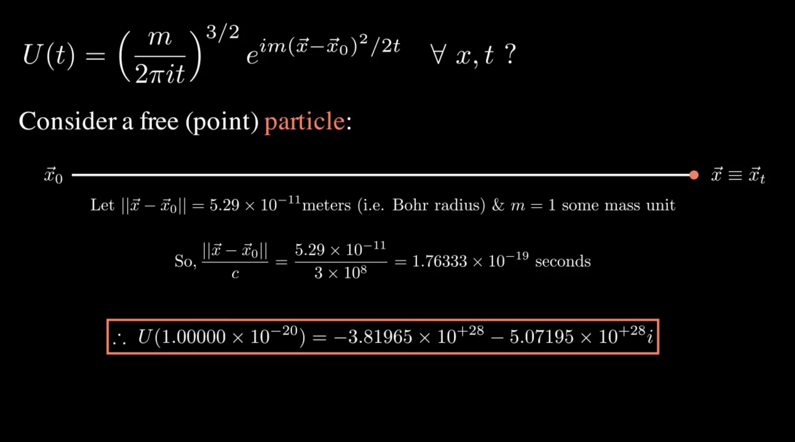
Consider the amplitude for a free particle to propagate from $\vec{x_{0}}$ to $\vec{x}$: $$ \begin{align*} U(t) = \braket{\vec{x} \vert e^{-i H t} \vert \vec{x}_{0}} \end{align*} $$ In the nonrelativisitic quantum mechanics, we have $E = \frac{\vec{p}^{2}}{2m} \equiv \frac{\vec{p}\cdot \vec{p}}{2m}$ (we will replace Hamiltonian operator by its eigen value), so
$$ \begin{aligned} U(t) &= \braket{\vec{x} \vert e^{-i ( \frac{\vec{p}^{2}}{2m}) t} \vert \vec{x}_{0}} \\ &= \text{Using \href{https://en.wikipedia.org/wiki/Orthonormal_basis}{completeness relation}, } \int \frac{d^{3} \vec{p}}{(2\pi)^{3}} \ket{\vec{p}}\bra{\vec{p}} = \mathbb{\hat{1}} \\ &= \int \frac{d^{3} \vec{p}}{(2\pi)^{3}} \braket{\vec{x} \vert e^{-i ( \frac{\vec{p}^{2}}{2m}) t} \ket{\vec{p}}\bra{\vec{p}}\vert \vec{x}_{0}} \\ &= \frac{1}{(2\pi)^{3}} \int d^{3}\vec{p} ~ e^{-i ( \frac{\vec{p}^{2}}{2m}) t} \braket{\vec{x} \vert \vec{p}} \braket{\vec{x}_{0} \vert \vec{p}}^{\dagger} \\ &\hspace{0.5cm} \text{where, } e^{-i ( \frac{\vec{p}^{2}}{2m}) t} \text{ is just a number.} \\ &= \text{Using } \braket{\vec{x} \vert \vec{p}} = e^{i \vec{p}\cdot \vec{x}}.\\ &= \frac{1}{(2\pi)^{3}} \int d^{3}\vec{p} ~ e^{-i ( \frac{\vec{p}^{2}}{2m}) t} e^{i \vec{p}\cdot (\vec{x} - \vec{x}_{0})}. \\ &= \text{Using Gaussian integral property}, \int_{-\infty}^{\infty} e^{-a x^{2} + bx + c} ~dx = \sqrt{\frac{\pi}{a}} e^{\frac{b^{2}}{4a} + c}. \\ &= \frac{1}{(2\pi)^{3}} \left(\sqrt{\frac{\pi}{\frac{i t}{2m}}}\right)^{3} ~ \exp\left(\frac{i^{2} (\vec{x} - \vec{x}_{0})^{2}}{4 (\frac{it}{2m})}\right) \\ &= (2\pi)^{3/2 - 3} \left(\frac{m}{i t} \right)^{3/2} \exp\left( \frac{i^{\cancel{2}} (\vec{x} - \vec{x}_{0})^{2}~2m}{4 \cancel{i} t}\right) \\ &= \left(\frac{m}{2\pi i t} \right)^{3/2} e^{i m (\vec{x} - \vec{x}_{0})^{2}/2t}. \end{aligned} $$
Some notes on completeness relations from a functional analysis point of view
Completeness relation allows us to define the inner product. Let’s understand it with an example using position space. It can be done in momentum space as well.
$\rightarrow$ For a single free particle moving in $n$-dimensional Euclidean (flat) manifold $\mathbb{R}^{n}$, we can have a complete orthonormal set of position basis vectors $\{\ket{x}\}$. So, we can define
$$ \begin{aligned} \braket{x \vert y} &= \delta(x, y), \\ \int_{\mathbb{R}^{n}} d^{n}x \ket{x}\bra{x} &= \mathbb{\hat{1}}. \end{aligned} $$
We can identify the Hilbert space $\mathcal{H}$ of such a system with the square-integrable complex-valued functions $L^{2}(\mathbb{R}^{n}, \mathbb{C})$ with the inner product
$$ \begin{aligned} \braket{\phi \vert \psi} &= \bra{\phi}\mathbb{\hat{1}}\ket{\psi} \\ &= \bra{\phi} \int_{\mathbb{R}^{n}} d^{n}x \ket{x}\bra{x} \ket{\psi} \\ \therefore \braket{\phi \vert \psi} &= \int_{\mathbb{R}^{n}} d^{n}x ~\phi_x \psi^{*}_{x} \end{aligned} $$
where $\phi_{x} \equiv \phi(x) := \braket{\phi \vert x}$ is the position basis coefficient, and same for $\psi_{x}$. Thus, $\psi^{*}_{x} = (\braket{\psi \vert x})^{*} = \braket{x \vert \psi}$. The unique existence of their spaces is guaranteed by the Riesz representation theorem.
I showed you how the completeness relation is used to define the inner product. It was possible because the position basis localized the state of a particle. But, this naive notion of position basis is not viable for fields (or differential forms) in Riemannian manifold $(\mathcal{M}, g)$ where the metric $g$ is not necessarily flat. It would be out of the scope of this note to further discuss the issue but, I will at least give you short reason.
$\rightarrow$ Suppose our $\phi$ is a $k$-forms in the space of differentials $k$-forms $\Omega^{k}(\mathcal{M})$. Due to the Hodge duality, we can find $(n - k)$-forms $* \phi \in \Omega^{n - k}(\mathcal{M})$ such that $\phi \leftrightarrow *\phi$ where
$$ \begin{aligned} \phi &= \phi_{i_1 \ldots i_k} ~dx^{i_1}\wedge \ldots \wedge dx^{i_k},\\ *\phi &= (*\phi)_{i_{k+1} \ldots i_n} ~ dx^{i_{k+1}}\wedge \ldots \wedge dx^{i_n} \end{aligned} $$
with coefficients
$$ \begin{aligned} \phi_{i_1 \ldots i_p} \leftrightarrow (*\phi)_{i_{k+1} \ldots i_n} = \frac{\sqrt{g}}{(n - k)!} \epsilon_{i_1 \ldots i_n}~ g^{i_1 j _1}\ldots g^{i_k j_k} \phi_{i_1 \ldots i_k}. \end{aligned} $$
The duality is up to a sign. i.e. $\ast\ast\phi = (-1)^{k (n - k)} \phi$. The inner product of $k$-forms is defined as$$ \begin{aligned} (\phi, \psi) &= \int_{\mathcal{M}} {\color{red}\phi} \wedge * \psi \\ &= \text{Using above definitions, we get}\\ &\quad \int_{\mathcal{M}} {\color{red}\phi_{i_1 \ldots i_k} ~dx^{i_1}\wedge \ldots \wedge dx^{i_k}} \wedge (*\phi)_{i_{k+1} \ldots i_n} ~ dx^{i_{k+1}}\wedge \ldots \wedge dx^{i_n}\\ &= \int_{\mathcal{M}} \phi_{i_1 \ldots i_k} (*\phi)_{i_{k+1} \ldots i_n} ~dx^{i_1}\wedge \ldots \wedge dx^{i_k} \wedge dx^{i_{k+1}}\wedge \ldots \wedge dx^{i_n} \\ &= \int_{\mathcal{M}} \phi_{i_1 \ldots i_k} (*\phi)_{i_{k+1} \ldots i_n} ~dx^{i_1}\wedge \ldots \wedge dx^{i_n} \\ \end{aligned} $$
and has a tensorial structure. It’s not easy to define a localized field. So, it is an open question of how to define it. Fortunately, with the quantum field theory that we learn from this book, our background metric is flat. So, we don’t have to worry about this issue. But, in quantum gravity, it’s an important question!
13P4B2
This expression is nonzero for all $x$ and $t$, indicating that a particle can propagate between any two points in an arbitrarily short time. In a relativistic theory, this conclusion would signal a violation of causality.
Just for fun!
To see the output of the below script in the output cell in Jupyter Notebook, you need to add
%%manim QFT13P4B2at the top of the cell.
# Require: manim. See https://docs.manim.community/en/stable/installation/conda.html
# Usage: manim QFT13P4B2.py QFT13P4B2
# Usage to generate medium quality gif: manim -qm --format=gif QFT13P4B2.py QFT13P4B2

from manim import *
import numpy as np

class QFT13P4B2(Scene):
  def construct(self):
    # Write the U(t)
    equation = MathTex("U(t) = \\left(\\frac{m}{2\\pi i t}\\right)^{3/2} e^{i m (\\vec{x} - \\vec{x}_{0})^{2}/2t} \\quad \\forall~ x, t~?")
    self.play(Write(equation))

    # Move the U(t) to the upper left corner
    self.play(equation.animate.to_corner(UL))

    # Write a text
    particle_type = Text("Consider a free (point) particle:", t2c={'particle':RED}).scale(0.7).next_to(equation, 2*DOWN).shift(1.5*LEFT)
    self.play(Write(particle_type))

    # Show how the particles moves from x_0 to x where white line is the displacement.
    free_particle = Dot(color=RED).next_to(particle_type, 2.5*DOWN).shift(2*LEFT)

    initial_position = MathTex("\\vec{x}_{0}").next_to(free_particle, 0.1*LEFT).scale(0.7)  # label the initial position
    self.play(Write(initial_position))

    particle_path= VMobject()
    particle_path.set_points_as_corners([free_particle.get_center(), free_particle.get_center()])

    def update_particle_path(particle_path):
      previous_particle_path = particle_path.copy()
      previous_particle_path.add_points_as_corners([free_particle.get_center()])
      particle_path.become(previous_particle_path)

    particle_path.add_updater(update_particle_path)

    self.add(particle_path, free_particle)
    self.play(free_particle.animate.shift(11*RIGHT))

    final_position = MathTex("\\vec{x}\\equiv\\vec{x}_t").next_to(free_particle, 0.1*RIGHT).scale(0.7)  # label the final position
    self.play(Write(final_position))

    # Define the distance travelled by the particle. Assume Bohr radius
    distance_travel = MathTex("\\text{Let } ||\\vec{x}-\\vec{x}_{0}|| = 5.29 \\times 10^{-11}\\text{meters (i.e. Bohr radius) \\& } m = 1 \\text{ some mass unit}").next_to(particle_path, DOWN).scale(0.6)
    self.play(Write(distance_travel))

    # Evaluate the ratio (x - x_0)/c
    x_c_ratio = MathTex("\\text{So}, \\frac{||\\vec{x}-\\vec{x}_{0}||}{c} = \\frac{5.29 \\times 10^{-11}}{3 \\times 10^8} = 1.76333 \\times 10^{-19}\\text{ seconds}").next_to(distance_travel, DOWN).scale(0.6)
    self.play(Write(x_c_ratio))

    # Write again the U(t) with t < (x - x_0)/c
    equation_t = MathTex("\\text{So, taking } t < \\frac{||\\vec{x}-\\vec{x}_{0}||}{c} \\text{ in } U(t) = \\left(\\frac{m}{2\\pi i t}\\right)^{3/2} e^{i m (\\vec{x} - \\vec{x}_{0})^{2}/2t}")
    equation_t.next_to(x_c_ratio, 3*DOWN).scale(0.7)
    self.play(Write(equation_t))
    self.wait(.5)

    # Evaluate U(t) for t in [1e-18, 1e-20] < (x - x_0)/c
    t = np.linspace(1e-18, 1e-20, 15)
    U_t = (1/(2*np.pi*1j*t))**(3/2) * np.exp(1j * (5.29e-11)**2/(2*t))

    for i in range(0, len(t)):
      sign = "+" if U_t[i].imag >= 0 else "-"
      equation_te = MathTex("\\therefore~ U(" + str(f"{t[i]:.5e}".replace('e', ' \\times 10^{')) + "}" + ") = " + str(f"{U_t[i].real:.5e}".replace('e', ' \\times 10^{')) + "}" + sign + str(f"{abs(U_t[i].imag):.5e}".replace('e', ' \\times 10^{'))+ "}" + "i")
      equation_te.next_to(x_c_ratio, 3*DOWN).scale(0.7)

      self.play(Transform(equation_t, equation_te), run_time=.5)
      framebox = SurroundingRectangle(equation_te, buff=0.1, color=RED)

      if i == 0:
        self.play(Create(framebox))

      self.remove(equation_te)
In special relativity, any motion of a particle from $\vec{x}_0$ to $\vec{x}$ in a time $t$ faster than the speed of light violates causality (i.e. $t < \frac{||\vec{x} - \vec{x}_0||}{c}$ where $c$ is the speed of light). This is because there is another inertial frame of reference in which the particle arrives at $\vec{x}$ at a time earlier than the time at which it leaves $\vec{x}_0$. Since the propagator $U(t)$ is non-zero for $t < \frac{||\vec{x} - \vec{x}_0||}{c}$, this means that the same particle can be in two places at the same time. This is a violation of causality and is not allowed in special relativity theory. We will come back to this point later on pages 28-29 in the book.
13P4E8
… . In analogy with the non-relativistic case, we have
$$ \begin{aligned} U(t) &= \braket{\vec{x} \vert e^{-i t \sqrt{\vec{p}^{2} + m^{2}}} \vert \vec{x}_{0}} \\ &= \text{Using completeness relation, } \int \frac{d^{3} \vec{p}}{(2\pi)^{3}} \ket{\vec{p}}\bra{\vec{p}} = \mathbb{\hat{1}} \\ &= \int \frac{d^{3} \vec{p}}{(2\pi)^{3}} \braket{\vec{x} \vert e^{-i t \sqrt{\vec{p}^{2} + m^{2}}} \ket{\vec{p}}\bra{\vec{p}}\vert \vec{x}_{0}} \\ &= \frac{1}{(2\pi)^{3}} \int d^{3}\vec{p} ~ e^{-i t \sqrt{\vec{p}^{2} + m^{2}}} \braket{\vec{x} \vert \vec{p}} \braket{\vec{x}_{0} \vert \vec{p}}^{\dagger} \\ &= \text{Using } \braket{\vec{x} \vert \vec{p}} = e^{i \vec{p}\cdot \vec{x}}.\\ &= \frac{1}{(2\pi)^{3}} \int d^{3}\vec{p} ~ e^{-i t \sqrt{\vec{p}^{2} + m^{2}}} e^{i \vec{p}\cdot (\vec{x} - \vec{x}_{0})}. \end{aligned} $$
Before we proceed, we do a transformation of momentum space in spherical (also called polar) coordinates $(p, \theta, \phi)$, and the volume element spanning from $\vec{p}$ to $\vec{p} + d\vec{p}$, $\theta$ to $\theta + d\theta$ and $\phi$ to $\phi + d\phi$ is given by the determinant of the Jacobian matrix of partial derivatives. i.e.
$$ \begin{aligned} dV := d^{3} \vec{p} &= \left| \frac{\partial (p_x, p_y, p_z)}{\partial (\vec{p}, \theta, \phi)} \right| d\vec{p} ~d\theta~ d\phi\\ &= p^{2} \sin(\theta) d\vec{p} ~d\theta~ d\phi\\ \therefore d^{3}p &= d\phi \sin(\theta) d\theta ~p^{2} d\vec{p} \end{aligned} $$
Now,$$ \begin{aligned} U(t) &= \text{Using } \vec{p}.(\vec{x} - \vec{x}_{0}) = p | \vec{x} - \vec{x}_{0}| \cos(\theta), \\ &\hspace{0.5cm} \text{\& spherical coordinate in momentum space}\\ &= \frac{1}{(2\pi)^{3}}\int d\phi \sin(\theta) d\theta ~p^2 d\vec{p} ~ e^{-i t \sqrt{p^2 + m^2}} ~e^{i p | \vec{x} - \vec{x}_{0}| \cos(\theta)} \\ &= \frac{1}{(2\pi)^{3}} \left[ \int_{0}^{2\pi} d\phi \right] \int \sin(\theta) d\theta ~p^2 d\vec{p} ~ e^{-i t \sqrt{p^2 + m^2}} ~e^{i p | \vec{x} - \vec{x}_{0}| \cos(\theta)} \\ &= \frac{\cancel{2\pi}}{(2\pi)^{\cancel{3}}} \int d\vec{p} ~p^2 ~ e^{-i t \sqrt{p^2 + m^2}} \left[ \int_{0}^{\pi}\sin(\theta) d\theta ~e^{i p | \vec{x} - \vec{x}_{0}| \cos(\theta)} \right]\\ &= \text{Do change of variable: } \zeta = \cos(\theta) \implies -d\zeta = \sin(\theta) d\theta\\ &= \frac{1}{(2\pi)^{2}} \int d\vec{p} ~p^2 ~ e^{-i t \sqrt{p^2 + m^2}} \left[ (-1) \int_{1}^{-1} d\zeta~ e^{i p |\vec{x} - \vec{x}_{0}| \zeta} \right]\\ &= \text{Since, } \int dx ~ e^{a x} = \frac{e^{a x}}{a} + \text{constant}.\\ &= \frac{1}{(2\pi)^{2}} \int d\vec{p} ~p^{\cancel{2}} ~ e^{-i t \sqrt{p^2 + m^2}} (-1) \left[ \frac{e^{i p |\vec{x} - \vec{x}_{0}|\zeta}}{i \cancel{p} |\vec{x} - \vec{x}_{0}|} \right]_{-1}^{~~1}\\ &= \frac{1}{(2\pi)^{2} |\vec{x} - \vec{x}_{0}|} \int d\vec{p} ~p ~ e^{-i t \sqrt{p^2 + m^2}} \left( \frac{e^{i p |\vec{x} - \vec{x}_{0}|} - e^{-i p |\vec{x} - \vec{x}_{0}|}}{i}\right)\\ &= \text{Using } \sin(x) = \frac{e^{ix} - e^{-ix}}{2i}.\\ &= \frac{1}{(2\pi)^{2} |\vec{x} - \vec{x}_{0}|} \int d\vec{p} ~p ~ e^{-i t \sqrt{p^2 + m^2}} (2) \sin(p |\vec{x} - \vec{x}_{0}|)\\ &= \frac{1}{2 \pi^{2} |\vec{x} - \vec{x}_{0}|} \int_{0}^{\infty} d\vec{p} ~p \sin(p |\vec{x} - \vec{x}_{0}|) ~ e^{-i t \sqrt{p^2 + m^2}}. \end{aligned} $$
13P4B3S1
This integral can be evaluated explicitly in terms of Bessel functions. Using the integral formula given in “2007 - Gradshteyn, Rhyzik- Table of Integrals, Series and Products”, page 491, formula number 3.914 (6) to the final expression of 13P4E8: $$ \int_0^\infty x e^{-\beta \sqrt{\gamma^2 + x^2}} \sin(bx) dx = \frac{b \beta \gamma^2}{\beta^2 + b^2} K_{2}( \gamma \sqrt{\beta^2 + b^2}) $$ where $K_{2}$ is the modified Bessel function of the second kind.
Here, $x \implies p, \beta \implies i t, \gamma \implies m, b \implies |\vec{x} - \vec{x}_{0}|$, so we get
$$ \begin{aligned} U(t) &= \frac{1}{2 \pi^{2} \cancel{|\vec{x} - \vec{x}_{0}|}} \frac{\cancel{|\vec{x} - \vec{x}_{0}|} (i t) m^{2}}{(i t)^{2} + |\vec{x} - \vec{x}_{0}|^{2}} K_{2}(m \sqrt{(i t)^{2} + |\vec{x} - \vec{x}_{0}|^{2}}) \\ &= \frac{i t m^{2}}{2 \pi^{2} (|\vec{x} - \vec{x}_{0}|^{2} - t^{2})} K_{2}(m \sqrt{|\vec{x} - \vec{x}_{0}|^{2} - t^{2}}) \end{aligned} $$
13P4B3S2
… with looking at its asymptotic behavior for $x^2 \gg t^2$ (well outside the light-cone), using the method of stationary phase. The function $px - t \sqrt{p^{2} + m^{2}}$ has a stationary point at $p = imx/\sqrt{x^{2} - t^{2}}$. Plugging in this value for $p$, we find that, upto a rational function of $x$ and $t$, $$U(t) \sim e^{-m \sqrt{x^2 - t^2}}.$$
Instead of transforming the above integral (defined in 13P4E8) to momentum space, we can also use the idea of stationary phase approximation to evaluate the integral.
Our objective here is to evaluate the integral into the asymptotic expansion from a stationary phase point up to the leading term of the contribution. This is the main idea of the “method of stationary phase”.
Before proceeding, let’s briefly review the method of the stationary phase.
I will be following chapter 6 ("$h$-Transforms with Oscillatory Kernels") from the book “Bleistein, Handelsman - Asymptotic Expansions of Integrals”.
Method of Stationary Phase
We consider the asymptotic expansion (as $\lambda \to \infty$) of integral(s) of the form: $$ I(\lambda) = \int_{a}^{b} \exp\{i \lambda \phi(t)\}~ f(t)~dt $$ where $\phi(t) \in \mathbb{R}$ is the phase function and $f(t)$ is an amplitude function; similar like in the Fourier integral.
Don’t be confused $I(\lambda)$ with Riemann–Lebesgue lemma. But, this is a useful tool in QFT which we will see its usage later. For example, in asymptotic state calculation using LSZ reduction formula for computing S-matrix.
If $f$ and $\phi$ are infinitely differentiable ($C^{\infty}$), and $\phi$ is monotonic on $[a, b]$, then an infinite asymptotic expansion of the above integral $I(\lambda)$ can be obtained via the integration-by-parts procedure. If the first derivative of $\phi$ vanishes at $c$ then, $c$ is a stationary point of $\phi$.
If the derivative of a function $\phi$ at point $c$ is equal to zero or undefined then, such a point is called critical point.
Now, let’s apply the above idea to our problem. We have,
$$ U(t) = \frac{1}{(2\pi)^3} \int d^{3}p ~ e^{i\left(\textcolor{green}{\vec{p}\cdot \vec{x} - t \sqrt{p^{2} + m^{2}}}\right)} ~e^{-i \vec{p}\cdot\vec{x}_{0}}, $$ the phase function of $U(t)$ is, $\phi(\vec{p}) = \textcolor{green}{\vec{p}\cdot \vec{x} - t \sqrt{p^{2} + m^{2}}}$.
To be consistent with the book’s text, we use $p$ instead of $c$ to denote the stationary point (i.e. $\vec{p}$ is variable, and $p$ is a point for evaluation). The stationary point can be achieved by solving $\left.\frac{d\phi(\vec{p})}{d\vec{p}} \right\vert_{\vec{p} = p} = 0$. See the “vector derivative cheat sheet” if you’re reluctant to do it. We proceed
$$ \begin{aligned} &\left.\frac{d\phi(\vec{p})}{d\vec{p}} \right\rvert_{\vec{p} = p} = 0\\ \text{or, }& x - \frac{t}{\cancel{2}} (p^2 + m^2)^{\frac{1}{2} - 1} \cancel{2}p = 0 \\ \text{or, }& x - \frac{t p}{\sqrt{p^2 + m^2}} = 0 \\ \text{or, }& x\sqrt{p^2 + m^2} = tp \\ \text{or, }& x^{2} (p^2 + m^2) = t^2 p^2 \\ \text{or, }& p^{2}(x^2 - t^2) = -x^2 m^2 \\ \therefore ~&~ p = i m x / \sqrt{x^2 - t^2} \end{aligned} $$
such that $x > t$. Since we want to do asymptotic expansion, we fine-tune $p$ such that $(x^{2} - t^{2}) \to \infty \implies x^2 \gg t^2$. This means the asymptotic expansion holds only when $x^2 \gg t^2$. The inequality ($\gg$) can be accounted for by re-defining $\phi$ as new $\phi := \lambda \phi$ (see below). I’m using the same symbol $\phi$ for new and old $\phi$ to account for inequality. Note that it does not influence the calculation because we want to see if the observable exists well outside the light-cone. Thus, the new $\phi$ will have a rapid oscillation. So, the $I_{p}(\lambda)$ becomes $I_{p}$ such that
$$ \boxed{I \approx \exp\{i \phi(p)\} f(p) \sqrt{\frac{2\pi}{|\phi^{\prime\prime}(p)|}} \exp\left\{\frac{\pi i \mu}{4}\right\}}. $$
Keep in mind that we are only going to compute $\left.\phi(\vec{p})\right\vert_{\vec{p}=p}$ and we show $U(t)$ does not vanish (which we already know from 13P4E8). Let’s move forward,
$$ \begin{aligned} \left.\phi(\vec{p})\right\vert_{\vec{p}=p} &= \htmlId{redefine-phi-lambda-phi}{p\cdot \vec{x} - t \sqrt{p^{2} + m^{2}}}\\ &= \frac{im\textcolor{blue}{\vec{x}}}{\sqrt{x^2 - t^2}}\cdot \textcolor{blue}{\vec{x}} - t\sqrt{\left( \frac{\textcolor{red}{i}m\vec{x}}{\sqrt{x^2 - t^2}}\right)^2 + m^2} \\ &= \frac{im \textcolor{blue}{x^2}}{\sqrt{x^2 - t^2}} - t \sqrt{\frac{\textcolor{red}{-}m^{2}x^{2}}{x^2 - t^2} + m^2} \\ &= \frac{im \textcolor{blue}{x^2}}{\sqrt{x^2 - t^2}} - t \sqrt{\frac{-\cancel{m^{2}x^{2}} + \cancel{m^{2}x^{2}} - m^{2}t^{2}}{x^{2} - t^{2}}} \\ &= \frac{imx^{2} - t (imt)}{\sqrt{x^{2} - t^{2}}} \\ &= \frac{im \cancel{(x^2 - t^2)}}{\cancel{\sqrt{x^2 - t^2}}}\\ &= i m \sqrt{x^2 - t^2}\\ &= \text{Redefine $\phi(p) \to \lambda\phi(p)\mid x^2 \gg t^2 \Harr \lambda \to \infty$ }\\ \therefore \exp\left\{i\phi(p)\right\} &= \exp\left\{- m \sqrt{x^2 - t^2}\right\}. \end{aligned} $$
We get $$ U(t) \sim e^{- m \sqrt{x^2 - t^2}}. $$Thus the propagation amplitude is small but nonzero outside the light-cone, and causality is still violated.
Noether Theorem
17E(2.11)-(2.12)
Consider infinitesimal form $\mathcal{L}(x) \to \mathcal{L^{\prime}}(x) = \mathcal{L}(x) + \alpha \Delta\mathcal{L}(x)$. Note that $\mathcal{L}(x)$ and $\mathcal{L}$ mean the same. So, $\alpha\Delta\mathcal{L} = \mathcal{L^{\prime}} - \mathcal{L} := \delta \mathcal{L}$. We can write:
$$ \begin{aligned} \alpha\Delta\mathcal{L} &= \delta\mathcal{L} \\ &= \text{Using the definition of the partial derivative.} \\ &= \frac{\partial \mathcal{L}}{\partial \phi} \delta\phi + \left(\frac{\partial \mathcal{L}}{\partial (\partial_{\mu}\phi)} \right) \delta(\partial_{\mu}\phi) \\ &= \text{Using eqn (2.9) i.e. } \delta\phi = \alpha\Delta\phi \text{ and } \delta(\partial_{\mu}\phi) = \partial_{\mu} (\delta\phi) = \partial_{\mu}(\alpha\Delta\phi) \\ &= \frac{\partial \mathcal{L}}{\partial \phi} (\alpha\Delta\phi) + {\color{red} \left(\frac{\partial \mathcal{L}}{\partial (\partial_{\mu}\phi)} \right) \partial_{\mu}(\alpha\Delta\phi)} \\ &= \text{Using chain rule in the red colored equation.} \\ &= \alpha \frac{\partial \mathcal{L}}{\partial \phi} (\Delta\phi) + {\color{red} \partial_{\mu}\left(\frac{\partial \mathcal{L}}{\partial (\partial_{\mu}\phi)} (\alpha\Delta\phi) \right) - \partial_{\mu}\left( \frac{\partial \mathcal{L}}{\partial (\partial_{\mu}\phi)} \right) (\alpha\Delta\phi)} \\ &= \alpha \partial_{\mu}\left( \frac{\partial \mathcal{L}}{\partial (\partial_{\mu}\phi)} \Delta\phi \right) + \alpha \left[ {\color{green}\frac{\partial \mathcal{L}}{\partial \phi} - \partial_{\mu}\left( \frac{\partial \mathcal{L}}{\partial (\partial_{\mu}\phi)} \right)} \right] \Delta\phi \quad (2.11) \\ &= \text{Green colored equation is EOM (2.3) equals to 0.} \\ &= \alpha \partial_{\mu}\left( \frac{\partial \mathcal{L}}{\partial (\partial_{\mu}\phi)} \Delta\phi \right) \end{aligned} $$
Comparing the above result with eqn (2.10). We get $\Delta\mathcal{L} = \partial_{\mu}\mathcal{J}^{\mu}(x)$. i.e.
$$ \begin{aligned} \partial_{\mu}\mathcal{J}^{\mu}(x) &= \partial_{\mu}\left( \frac{\partial \mathcal{L}}{\partial (\partial_{\mu}\phi)} \Delta\phi \right) \\ \therefore \partial_{\mu} \left( {\color{blue}\frac{\partial \mathcal{L}}{\partial (\partial_{\mu}\phi)} \Delta\phi - \mathcal{J}^{\mu}} \right) &:= \partial_{\mu}{\color{blue}j^{\mu}(x)} = 0. \quad (2.12) \end{aligned} $$
The blue-colored equation is defined as current. The eqn (2.12) means the divergence of current vanishes.If the symmetry involves more than one field (say $\phi_{1}, \phi_{2}, \ldots, \phi(n)$), the first term of the eqn (2.12) for $j^{\mu}(x)$ should be replaced by a sum of such terms, one for each field. i.e.
$$ \begin{aligned} \displaystyle\sum_{\mu=0}^3 \frac{\partial \mathcal{L}}{\partial (\partial_{\mu}\phi)} \Delta\phi &\xrightarrow[\text{by}]{\text{Replace}} \displaystyle\sum_{i=1}^n \displaystyle\sum_{\mu=0}^3\frac{\partial \mathcal{L}}{\partial (\partial_{\mu}\phi_{i})} \Delta\phi_{i} \\ &\equiv \text{In Einstein's convention, } \frac{\partial \mathcal{L}}{\partial (\partial_{\mu}\phi_{i})} \Delta\phi_{i} \end{aligned} $$
Note: Einstein’s convention means we sum over repeated indices. These indices we call dummy indices, as you can relabel them as you like. We will use Einstein’s convention most of the time unless it needs explicit form.
18P2B0
… so we conclude that the current $j^{\mu} = \partial^{\mu}\phi$.
Given $\mathcal{L} = \frac{1}{2}(\partial_{\mu}\phi)^{2} \equiv \frac{1}{2} (\partial_{\mu}\phi)(\partial^{\mu}\phi)$ and $\phi \to \phi + \alpha$ so deformation of field $\Delta\phi = 1$ i.e. we only rescale our field $\phi$ by scale $\alpha$. Our Lagrangian is scale invariance (a symmetry) because $\partial_{\mu}\alpha = 0$. Thus, we demand one conservation law because of Noether’s theorem. Note we assume $\mathcal{J}^{\mu} = 0$. Hence, the current is
$$ \begin{aligned} j^{\mu} &= \frac{\partial \mathcal{L}}{\partial (\partial_{\mu}\phi)} \Delta\phi - \mathcal{J}^{\mu} \\ &= \frac{\partial \mathcal{L}}{\partial (\partial_{\mu}\phi)} \\ &= \frac{1}{2}\frac{\partial \left( (\partial_{\mu}\phi)(\partial^{\mu}\phi) \right)}{\partial (\partial_{\mu}\phi)} \\ &= \frac{1}{2} \left[ \frac{\partial (\partial_{\mu}\phi)}{\partial (\partial_{\mu}\phi)} (\partial^{\mu}\phi) + (\partial_{\mu}\phi) \frac{\partial ({\color{green}\partial^{\mu}}\phi)}{\partial (\partial_{\mu}\phi)} \right] \\ &= \text{Using } {\color{green}\partial^{\mu} = g^{\mu\nu} \partial_{\nu}}. \\ &= \frac{1}{2} \left[ \partial^{\mu}\phi + (\partial_{\mu}\phi) {\color{green}g^{\mu\nu}} \frac{\partial ({\color{green}\partial_{\nu}}\phi)}{\partial (\partial_{\mu}\phi)}\right] \\ &= \frac{1}{2} \left[ \partial^{\mu}\phi + (\partial_{\mu}\phi) g^{\mu\nu} \delta^{\nu}_{\mu} \right] \\ &\quad \text{where } \frac{\partial (\partial_{\nu}\phi)}{\partial (\partial_{\mu}\phi)} = \delta^{\nu}_{\mu} := \text{ Kronecker delta}. \\ &= \frac{1}{2} \left[ \partial^{\mu}\phi + (\partial_{\mu}\phi) g^{\mu\nu} \delta^{\nu}_{\mu} \right] \\ &= \frac{1}{2} \left[ \partial^{\mu}\phi + {\color{red}(\partial^{\nu}\phi) \delta^{\nu}_{\mu}} \right] \\ &= \frac{1}{2} \left[ \partial^{\mu}\phi + {\color{red}\partial^{\mu}\phi} \right] \\ \therefore j^{\mu} &= \partial^{\mu} \phi. \end{aligned} $$
18P2E(2.15)-(2.16)
Given the Lagrangian for complex scalar field, $$\mathcal{L} = |\partial_{\mu}\phi |^{2} - m^{2}|\phi|^{2} \equiv (\partial_{\mu}\phi)(\partial^{\mu}\phi^{*}) - m^{2} \phi\phi^{*} \quad (2.14)$$ … the transformation $\phi \to e^{i\alpha}\phi$; for an infinitesimal transformation with $\mathcal{O}(\alpha^{2})$ we have
$$ \begin{aligned} \phi \to \phi' &= e^{i\alpha} \phi \\ &= \text{Under infinitesimal transformation}\\ &= (1 + i\alpha)\phi \\ &= \phi + i\alpha\phi \end{aligned} $$
Similarly,$$ \begin{aligned} \phi^{*} \to {\phi^{*}}' &\equiv (\phi')^{*} = (e^{i\alpha} \phi)^{*} = e^{-i\alpha} \phi^{*} \\ &= \text{Under infinitesimal transformation}\\ &= (1 - i\alpha)\phi^{*} \\ &= \phi^{*} - i\alpha\phi^{*} \end{aligned} $$
Comparing above results with $\phi \to \phi' = \phi + \alpha\Delta\phi$ and $\phi \to {\phi^{*}}' = \phi^{*} + \alpha\Delta\phi^{*}$ respectively. We get $\Delta\phi = i\phi$ and $\Delta\phi^{*} = -i\phi^{*}\quad (2.15)$.… conserved Noether current is
$$ \begin{aligned} j^{\mu} &= \displaystyle\sum_{i=1}^n \frac{\partial \mathcal{L}}{\partial (\partial_{\mu}\phi_{i})} \Delta\phi_{i} - \mathcal{J}^{\mu} \\ &\quad \text{Since, } \mathcal{J}^{\mu} = 0 \\ &= {\color{red}\frac{\partial \mathcal{L}}{\partial (\partial_{\mu}\phi)} \Delta\phi} + {\color{green}\frac{\partial \mathcal{L}}{\partial (\partial_{\mu}\phi^{*})} \Delta\phi^{*}} \\ &= {\color{red} \frac{\partial [(\partial_{\mu}\phi)(\partial^{\mu}\phi^{*}) - m^{2} \phi\phi^{*}]}{\partial (\partial_{\mu}\phi)}} (i\phi) + {\color{green} \frac{\partial [(\partial_{\mu}\phi)(\partial^{\mu}\phi^{*}) - m^{2} \phi\phi^{*}]}{\partial (\partial_{\mu}\phi^{*})}} (-i\phi^{*}) \\ &= \text{Note that } \frac{\partial (\phi\phi^{*})}{\partial (\partial_{\mu}\phi)} = 0. \text{ Also, $\phi$ and $\phi^{*}$ are independent fields.}\\ &\hspace{.5cm} \text{Using \href{https://en.wikipedia.org/wiki/Product_rule}{Leibniz product rule.}} \\ &= {\color{red} (\partial^{\mu}\phi^{*}) (i\phi)} - {\color{green} (\partial_{\mu}\phi) g^{\mu\nu}\frac{\partial (\partial_{\nu}\phi^{*})}{\partial (\partial_{\mu}\phi^{*})} (i\phi^{*})} \\ &= i [(\partial^{\mu}\phi^{*})\phi - \phi^{*} (\partial_{\mu}\phi)g^{\mu\nu}\delta^{\nu}_{\mu}]\\ &= i[(\partial^{\mu}\phi^{*})\phi - \phi^{*}(\partial^{\mu}\phi)] \quad (2.16) \end{aligned} $$
18P2B3
… the divergence of this current vanishes by using the Klein-Gordon equation. i.e.
$$ \begin{aligned} \partial_{\mu} j^{\mu} &= i[\partial_{\mu}\{(\partial^{\mu}\phi^{*})\phi\} - \partial_{\mu}\{\phi^{*}(\partial^{\mu}\phi)\}] \\ &= \text{Using product rule.} \\ &= i [(\partial_{\mu}\partial^{\mu} \phi^{*})\phi + \cancel{(\partial^{\mu}\phi^{*})(\partial_{\mu}\phi)} - \cancel{(\partial_{\mu}\phi^{*})(\partial^{\mu}\phi)} - \phi^{*}(\partial_{\mu}\partial^{\mu}\phi)] \\ &= \partial_{\mu}\partial^{\mu} \equiv \partial^{\mu}\partial_{\mu} := \square^{2} \text{ called as d'Alembertian, and} \\ &\quad (\partial^{\mu}\phi^{*})(\partial_{\mu}\phi) \equiv (\partial_{\mu}\phi^{*})(\partial^{\mu}\phi) \equiv |\partial_{\mu}\phi|^{2}. \\ &= i [(\square^{2}\phi^{*})\phi - \phi^{*}(\square^{2}\phi)] \\ &= \text{Using Euler-Lagrange EOM: } \\ &\quad\quad \frac{\partial \mathcal{L}}{\partial \phi} - \partial_{\mu}\left( \frac{\partial \mathcal{L}}{\partial (\partial_{\mu}\phi)} \right) = 0 \\ &\quad\quad \text{or, } -m^{2}\phi^{*} - \partial_{\mu}\partial^{\mu}\phi^{*} = 0 \\ &\quad\quad \therefore (\square^{2} + m^{2})\phi^{*} = 0 \text{ is Klein-Gordon eqn.}\quad (2.7) \\ &\quad\quad\text{or, } \square^{2}\phi^{*} = -m^{2}\phi^{*}\quad \times \phi \text{ both sides} \\ &\quad\quad \therefore (\square^{2}\phi^{*})\phi = -m^{2}\phi^{*}\phi \equiv -m^{2} |\phi|^{2}\\ &\quad \text{Similarly, } \\ &\quad\quad \frac{\partial \mathcal{L}}{\partial \phi^{*}} - \partial_{\mu}\left( \frac{\partial \mathcal{L}}{\partial (\partial_{\mu}\phi^{*})} \right) = 0 \\ &\quad\quad \text{or, } -m^{2}\phi - \partial_{\mu} \left[ \partial_{\mu}\phi \frac{\partial(\partial^{\mu}\phi^{*}) }{\partial (\partial_{\mu}\phi^{*})} \right] = 0 \\ &\quad\quad \text{or, } -m^{2}\phi - \partial_{\mu} \left[ \partial_{\mu}\phi ~g^{\mu\nu}~ \frac{\partial (\partial_{\nu}\phi^{*})}{\partial (\partial_{\mu}\phi^{*})}\right] = 0 \\ &\quad\quad \text{or, } -m^{2}\phi - \partial_{\mu}[\partial^{\nu}\phi~ \delta^{\nu}_{\mu}] = 0 \\ &\quad\quad \text{or, } -m^{2}\phi - \partial_{\mu}\partial^{\mu}\phi = 0 \\ &\quad\quad \text{or, } \square^{2}\phi = -m^{2}\phi \quad \times \phi^{*} \text{ from left} \\ &\quad\quad \therefore \phi^{*}\square^{2}\phi = -m^{2}|\phi|^{2}\\ &\quad \text{Substituting the acquired identities.} \\ &= i[-\cancel{m^{2}|\phi|^{2}} + \cancel{m^{2}|\phi|^{2}}] \\ &= 0. \end{aligned} $$
Note: we’re using the d’Alembertian operator (or simply d’Alembertian) as $\square^{2}$ but other books might write just $\square$.
19E(2.17)-(2.19)
Noether’s theorem can also be applied to spacetime transformations such as translations and rotations. We can describe the infinitesimal translation $$x^{\mu} \to x^{\mu} - a^{\mu}$$ alternatively as a transformation of the field configuration $$\phi(x) \to \phi(x + a) = \phi(x) + a^{\mu}\partial_{\mu}\phi(x).$$
This and previously $(2.9)$, we did infinitesimal transformations of the fields as a Taylor expansion up to the first order in fields and their derivatives.
We can write $\delta\phi(x) := \phi(x + a) - \phi(x) = a^{\mu}\partial_{\mu}\phi(x)$.
The Lagrangian is also a scalar, so it must transform in the same way: $$\mathcal{L} \to \mathcal{L} + a^{\mu}\partial_{\mu}\mathcal{L} \equiv \mathcal{L} + a^{\nu} \partial_{\mu}(\delta^{\mu}{}_{\nu}\mathcal{L}).$$
$$ \begin{align*} a^{\nu} \partial_{\mu}(\delta^{\mu}{}_{\nu}\mathcal{L})&= \delta \mathcal{L}(x) \\ &= \text{Since, } \mathcal{L} \equiv \mathcal{L}(\phi(x), \partial_{\mu}\phi(x)) \text{. we write}\\ &\hspace{.5cm} \frac{\partial\mathcal{L}}{\partial\phi} \delta\phi + \left( \frac{\partial\mathcal{L}}{\partial(\partial_{\mu}\phi)} \right) {\color{green}\delta(\partial_{\mu} \phi)} \\ &= \frac{\partial\mathcal{L}}{\partial\phi} \delta\phi + \left( \frac{\partial\mathcal{L}}{\partial(\partial_{\mu}\phi)} \right) {\color{green}\partial_{\mu}(\delta\phi)} \\ &= \text{Substituting } \delta\phi = a^{\nu}\partial_{\nu}\phi, \text{ and using Leibniz product rule:}\\ &\hspace{.5cm} \frac{\partial\mathcal{L}}{\partial\phi} (a^{\nu}\partial_{\nu}\phi) + \partial_{\mu} \left( \frac{\partial\mathcal{L}}{\partial(\partial_{\mu}\phi)} (a^{\nu}\partial_{\nu}\phi) \right) - \partial_{\mu} \left( \frac{\partial\mathcal{L}}{\partial(\partial_{\mu}\phi)}\right) (a^{\nu}\partial_{\nu}\phi)\\ &= \text{Since, } a^{\nu} \text{ is just a constant, i.e. not a function of } x. \text{ So,}\\ &\hspace{.5cm} \text{We can take } a^{\nu} \text{ out of the derivative. We get}\\ &\hspace{.5cm} a^{\nu} {\color{red}\left[ \frac{\partial\mathcal{L}}{\partial\phi} - \partial_{\mu} \left(\frac{\partial\mathcal{L}}{\partial(\partial_{\mu}\phi)} \right) \right]} \partial_{\nu}\phi + a^{\nu }\partial_{\mu} \left( \frac{\partial\mathcal{L}}{\partial (\partial_{\mu} \phi)} \partial_{\nu}\phi \right)\\ &= \text{{\color{red}Red color expression is zero} due to Euler-Lagrange eqn.}\\ \therefore a^{\nu} &\partial_{\mu}\left[ {\color{blue}\frac{\partial\mathcal{L}}{\partial(\partial_{\mu}\phi)} \partial_{\nu}\phi - \delta^{\mu}{}_{\nu}\mathcal{L}} \right]= 0.\\ \end{align*} $$
The blue color expression is defined as Noether conserved 4-currents ${\color{blue} T^{\mu}{}_{\nu}}$.
$$ T^{\mu}{}_{\nu} := \frac{\partial\mathcal{L}}{\partial(\partial_{\mu}\phi)} \partial_{\nu}\phi - \mathcal{L} \delta^{\mu}{}_{\nu} \quad (2.17) $$
This is precisely the stress-energy tensor, also called the energy-momemtum tensor, of the field $\phi$.
Now, we are going to prove equations $(2.18)$ (that Hamiltonian density $\mathcal{H}$ equals to $T^{00}$) and $(2.19)$ (that momentum density $\Pi$ times the velocity of the field $\phi$ equals to $T^{0i}$). We start from
$$ \begin{align*} T^{\mu\rho} \equiv g^{\rho\nu} T^{\mu}{}_{\nu} = g^{\rho\nu} \left( \frac{\partial\mathcal{L}}{\partial(\partial_{\mu}\phi)} \partial_{\nu}\phi - \mathcal{L} \delta^{\mu}{}_{\nu} \right). \end{align*} $$
Note that the metric tensor $g^{\rho\nu} := \text{diag}(+1, -1, -1, -1) \text{ else } 0$. So,
$$ \begin{align*} T^{00} &= g^{00} \left( {\color{green}\frac{\partial\mathcal{L}}{\partial(\partial_{0}\phi)}} \partial_{0}\phi - \mathcal{L} \delta^{0}{}_{0} \right) \\ &= \text{Substituting the canonical momentum } {\color{green}\pi := \frac{\partial\mathcal{L}}{\partial \dot{\phi}}} \text{ gives} \\ &\hspace{.5cm} {\color{green}\pi} \dot{\phi} - \mathcal{L} \\ &\hspace{.5cm} \text{is a \href{https://en.wikipedia.org/wiki/Legendre_transformation\#Analytical_mechanics}{Legendre transformation} for Hamiltonian formulation.}\\ &= \mathcal{H}. \end{align*} $$
The conserved charge associated with time translation (i.e. $x^{0} \to x^{0} - a^{0}$) is the Hamiltonian (i.e. total energy of the system): $$H = \int \mathcal{H} ~d^{3}x \equiv \int T^{00} ~d^{3}x. \quad (2.18)$$
Similarly,
$$ \begin{align*} T^{0i} &= g^{i\nu} \left( \frac{\partial\mathcal{L}}{\partial(\partial_{0}\phi)} \partial_{\nu}\phi - \mathcal{L} \delta^{0}{}_{i} \right) \\ &\hspace{.5cm} \text{Note that } \nu \in (0, 1, 2, 3) \text{ but, } i \in (1, 2, 3).\\ &= \text{For } \nu = i \implies g^{ii} = -1, \text{ but } i \neq \nu \implies g^{i\nu} = 0. \text{ So,}\\ &\hspace{.5cm} g^{ii}\left( {\color{green}\frac{\partial\mathcal{L}}{\partial \dot{\phi}}} \partial_{i}\phi - \mathcal{L} {\color{red}\delta^{0}{}_{i}} \right)\\ &= \text{Since, } {\color{red}\delta^{0}{}_{i} = 0}. \text{ So,}\\ &\hspace{.5cm} - {\color{green}\pi} \partial_{i}\phi \end{align*} $$
The conserved charges (phural due to 3 conserved charges) associated with spatial translations (i.e. $x^{i} \to x^{i} - a^{i}$) are the physical momenta (not to be confused with the canonical momentum): $$P^{i} = - \int \pi \partial_{i}\phi ~d^{3}x \equiv \int T^{0i} ~d^{3}x. \quad (2.19)$$
Permalink at https://www.physicslog.com/physics-notes/qft/the-klein-gordon-field
Published on Aug 24, 2021
Last revised on Dec 18, 2023
References