Convergence and Stability

Join the Discussion
← Preface
← Sources of Numerical Errors
→ Power Method

Highlights

Convergence

In this topic, we will discuss the convergence and stability of iterative algorithms.

Convergence

We expect numerical algorithms should converge to the exact solution $x_{*}$. The iteration produces a sequence of approximations ${x_n}$. The sequence ${x_n}$ is said to converge to $x_{*}$ if $$\lim_{n\to\infty} x_n = x_{*}.$$ This suggests that we need to find a fixed point solution of the iteration method (i.e. $f(x_{*}) = x_{*}$ where $f(x_{*}) := x_{n}$).

Let’s understand using an example:

Consider a Logistic map: $x \ni [0, 1] \to f(x) := k x (1 - x) \in [0, 1] ~\forall~ k \in [0, 4]$.

Let’s compute the fixed point of above definition:

$$ \begin{aligned} x_{*} &= f(x_{*}) \\ &= k x_{*} (1 - x_{*}) \\ or,~ x_{*} (1 - k x_{*}) &= 0 \end{aligned} $$

Either $x_{*}$ = 0 or, $1 - k (1 - x_{*}) = 0 \implies x_{*} = 1 - \frac{1}{k}$.

The iteration equation of Logistic map is $x_{n+1} = k x_{n} (1 - x_{n})$. In non-linear dynamics,

the fixed point is 1-cycle, meaning that after each iteration, the value obtained from the map is the same. To find a fixed point, we solve $f(x) = x$.
2-cycle means that for every two iterations, the value obtained from the map is the same. To find a fixed point, we solve $f(f(x)) = x$.
and so on.

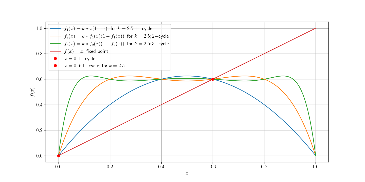
Let’s see an illustration of different cycles in the Logistic map for $k = 2.5 \implies x_{*} = 1 - \frac{1}{2.5} = 0.6$. If $x_{*} = 0.6$ for $k = 2.5$, then, $f_{n}(f_{n-1}(x_{*})) = \ldots = f_{3}(f_{2}(x_{*})) = f_{2}(f_{1}(x_{*})) = f_{1}(x_{*}) = 0.6$. Let’s see them numerically:

%matplotlib inline
import matplotlib.pyplot as plt
import numpy as np

k = 2.5
x = np.linspace(0, 1, 1000)
y1 = k * x*(1-x)
y2 = k * y1 * (1 - y1)
y3 = k * y2 * (1 - y2)
y = x

plt.plot(x, y1, label=r'$f_1(x) = k * x (1 - x)$, for $k = {}; 1-$cycle'.format(k))
plt.plot(x, y2, label=r'$f_2(x) = k * f_1(x) (1 - f_1(x))$, for $k = {}; 2-$cycle'.format(k))
plt.plot(x, y3, label=r'$f_3(x) = k * f_2(x) (1 - f_2(x))$, for $k = {}; 3-$cycle'.format(k))
plt.plot(x, y, label=r'$f(x) = x$; fixed point')
plt.plot(0, 0, 'ro', label=r'$x = 0; 1-$cycle')
plt.plot(1 - 1/k, 1 - 1/k, 'ro', label=r'$x = {}; 1-$cycle; for $k = {}$'.format(1 - 1/k, k))
plt.xlabel(r'$x$')
plt.ylabel(r'$f(x)$')
plt.legend()
# plt.savefig('logistic_map-n-cycles-k_2-5.png')
plt.show()

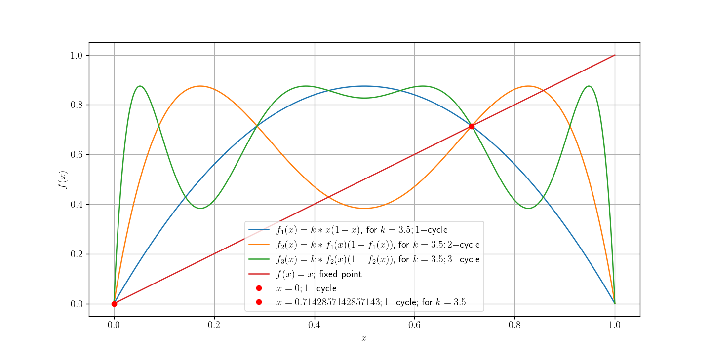
It shows all $f_{i}(x)$ have fixed points at $x = 0.6$! Let’s see another illustration of different cycles in Logistic map for $k = 3.5$:

%matplotlib inline
import matplotlib.pyplot as plt
import numpy as np

k = 3.5
x = np.linspace(0, 1, 1000)
y1 = k * x*(1-x)
y2 = k * y1 * (1 - y1)
y3 = k * y2 * (1 - y2)
y = x

plt.plot(x, y1, label=r'$f_1(x) = k * x (1 - x)$, for $k = {}; 1-$cycle'.format(k))
plt.plot(x, y2, label=r'$f_2(x) = k * f_1(x) (1 - f_1(x))$, for $k = {}; 2-$cycle'.format(k))
plt.plot(x, y3, label=r'$f_3(x) = k * f_2(x) (1 - f_2(x))$, for $k = {}; 3-$cycle'.format(k))
plt.plot(x, y, label=r'$f(x) = x$; fixed point')
plt.plot(0, 0, 'ro', label=r'$x = 0; 1-$cycle')
plt.plot(1 - 1/k, 1 - 1/k, 'ro', label=r'$x = {}; 1-$cycle; for $k = {}$'.format(1 - 1/k, k))
plt.xlabel(r'$x$')
plt.ylabel(r'$f(x)$')
plt.legend()
# plt.savefig('logistic_map-n-cycles-k_3-5.png')
plt.show()

For $k = 3.5$, it shows that $f_{2}(x)$ has more fixed points. If you increase $k$ more, you will see most of the $f_{i}(x)$ have more than one fixed point. This means the solution is not stable for greater values of $k$. The stability of a solution is the property of an iterative equation that tells us whether the solution will remain the same or change over iteration. Let’s see an animation of the stability of the solution for different values of $k$ in 1-cycle:

# Not to show any inline output
%matplotlib agg

import matplotlib.pyplot as plt
import numpy as np
import matplotlib.animation as animation
from IPython.display import Image, display

# lower dpi to make gif size smaller
plt.rcParams.update({
    "figure.dpi": 70
})

fig = plt.figure()
ax = fig.add_subplot(111)
ax.set_xlim(0, 100)
ax.set_ylim(0, 1)
ax.set_xlabel('$n$')
ax.set_ylabel(r'$x_n$')
ax.set_title(r'$1-$cycle for different values of $k$')

line, = ax.plot([], [], lw=2)

def init():
    line.set_data([], [])
    return line,

def animate(i):
    k = i/10
    x = 0.6
    n = np.arange(101)
    xn = [x]
    for i in np.arange(100):
      x = k * x*(1-x)
      xn.append(x)

    line.set_data(n, xn)
    ax.set_title('1-cycle for different values of k; k = {}'.format(k))
    return line,

ani = animation.FuncAnimation(fig, animate, init_func=init, frames=40, interval=300, blit=True)
ani.save('1-cycles-different-values-of-k.gif', writer='imagemagick', fps=10)

with open('1-cycles-different-values-of-k.gif','rb') as f:
  display(Image(data=f.read(), format='png', width=1000))

# set dpi to our default value i.e. 120. This is optional
plt.rcParams.update({
    "figure.dpi": 120
})

It shows for approx. $k < 3$, the solution is stable. For approx. $k > 3$, the solution becomes unstable, and for $k = 4$, the solution is chaotic.

Permalink at https://www.physicslog.com/cs-notes/nm/convergence-and-stability
Published on Feb 15, 2023
Last revised on Feb 16, 2023